#simplify polynomial expression
Explore tagged Tumblr posts
Visit Tumblr Blog
Explore Tumblr blogs with no restrictions, modern design and the best experience.
Last Seen Tumblr Blogs


Fun Fact
Premium Tumblr themes are available from anywhere between $9 to $49.
Text
Review Canceling


1 note
·
View note
Text
youtube
Theres this youtube video, and you dont need to watch it to understand the post (thumbnail is sufficient)
the video basically proves that z^n+1/z^n, where n is a power of 2, is always -1.
then he rewrites z²⁰²⁴+1/z²⁰²⁴ into products of expressions of that form where the exponents sum to 2024? and kinda skips over how it can be rewritten like that...
to check this, (in case multiplying the factors actually sums the exponents like that) i multiplied

out to get
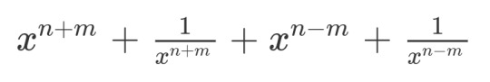
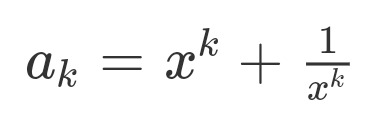
so if we say:
then the expanded equation simplifies to:
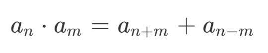
....which looks alot like a recursion relation if we set m=1 to get:
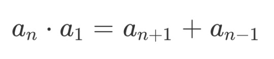
and since we know a_1=1 we get:

or, rearranging:
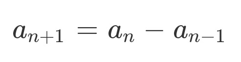
and if this is a recursion relation, we need one more term. a_0 is trivially 2, so generating the list to see some patterns:
0:2
1:1
2:-1
3:-2
4:-1
5:1
6:2
7:1
and it repeats! mod 6. 2024 ≡ 2 mod 6 so a_2024 = a_2 = -1 which is the answer the video got! good. it also gives a formula for all possible values of n! which is nice.
a few nice things:
a_n trivially equals a_-n, and we can see that in the pattern! the sequence from 0 to 6 is symmetric, so bringing that whole thing down so the 6 is at 0 is the same as reflecting it across 0!
powers of 2 are still -1 with this interpretation, as powers of 2 are always 2 or 4 mod 6! switching between the 2,
if you set a_1 to k, then the recursive formula is:
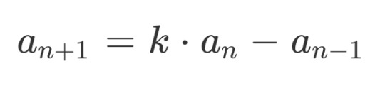
looking at a couple iterations, it looks like its always some sort of polynomial of k with every other power and the coefficients being some sort of choose-function esque thing...
3 notes
·
View notes
Text
Algebra - Introduction and Basic Formula
INTRODUCTION AND BASIC FORMULAS IN ALGEBRA
Algebra is the part of mathematics that helps to represent the problems or situations in the form of mathematical expressions. Algebraic formula are used to simplify the algebraic statement. Algebraic formulas are useful for resolving algebraic, quadratic, polynomials, trigonometry, probability, and more.
Introduction of Algebra
Algebra is the branch of mathematics in which arithmetical operations and formal manipulations are applied to abstract symbols rather than specific numbers. The notion that there exists such a distinct subdiscipline of mathematics, as well as the term algebra to denote it, resulted from a slow historical development. This article presents that history, tracing the evolution over time of the concept of the equation, number systems, symbols for conveying and manipulating mathematical statements, and the modern abstract structural view of algebra. For information on specific branches of algebra, see elementary algebra, linear algebra and modern algebra.
Algebraic Formula
Algebraic formulas are the combination of numbers and letters to form an equation or formula. The algebraic formula is a short quick formula to solve complex algebraic calculations.
Algebraic properties
The properties of algebra enable us to solve mathematical equations. Notice that these properties hold for addition and multiplication. These properties include the associative property, commutative property, distributive property, identity property, inverse property, reflexive property, symmetric property, and transitive property.
Algebraic Formula
a2 – b2 = (a – b)(a + b)
(a + b)2 = a2 + 2ab + b2
a2 + b2 = (a + b)2 – 2ab
(a – b)2 = a2 – 2ab + b2
(a + b + c)2 = a2 + b2 + c2 + 2ab + 2bc + 2ca
(a – b – c)2 = a2 + b2 + c2 – 2ab + 2bc – 2ca
(a + b)3 = a3 + 3a2b + 3ab2 + b3
( a + b )3 = a3 + b3 + 3ab(a + b)
(a – b)3 = a3 – 3a2b + 3ab2 – b3 or a3 – b3 – 3ab(a – b)
a3 – b3 = (a – b)(a2 + ab + b2)
a3 + b3 = (a + b)(a2 – ab + b2)
(a + b)4 = a4 + 4a3b + 6a2b2 + 4ab3 + b4
(a – b)4 = a4 – 4a3b + 6a2b2 – 4ab3 + b4
a4 – b4 = (a – b)(a + b)(a2 + b2)
a5 – b5 = (a – b)(a4 + a3b + a2b2 + ab3 + b4)
If n is a natural number an – bn = (a – b)(an-1 + an-2b+…+ bn-2a + bn-1)
If n is even (n = 2k), an + bn = (a + b)(an-1 – an-2b +…+ bn-2a – bn-1)
If n is odd (n = 2k + 1), an + bn = (a + b)(an-1 – an-2b +an-3b2…- bn-2a + bn-1)
(a + b + c + …)2 = a2 + b2 + c2 + … + 2(ab + ac + bc + ….)
Laws of Exponents (am)(an) = am+n ; (ab)m = ambm ; (am)n = amn
Properties of Algebra :
Commutative property:
Addition : a + b = b + a
Changing the order of addons does not change the sum.
Multiplication : a x b = b x a
Changing the order of the factor does not change the product.
Associative Property:
Addition : (a + b)+ c = a + (b + c)
Changing the grouping of the addends does not change the sum.
Multiplication : (a x b) xc = a x (b x c)
Changing the grouping of the factors does not change the product.
Distributive properties:
Addition : a × (b + c) = a × b + a × c
Multiplication : (a + b) × c = a × c + b × c
The distributive property states that multiplying each element by a single term and then adding and subtracting the products is the same as multiplying each component by a single term and then adding and subtracting the products.
Rule of multiplication over subtraction: p (q-r) = p*q – p*r
If p, q, and r, are all integers.
Left distributive law if p* (q-r) = (p * q) – (p*r)- and
Right distributive law if (p-q)*r = (p*r) – (q*r)-

What are the properties of Algebra?
Associative Property
Commutative Property
Distributive Property
Identity Property
Inverse Property
Reflexive Property
Symmetric Property
Transitive Property
Read more...
2 notes
·
View notes
Text
ACT Math Practice Tips for Mastering Every Section

The ACT Math section can feel like a high-pressure sprint: 60 questions in 60 minutes, covering everything from basic arithmetic to trigonometry. Whether you’re a math whiz or someone who breaks into a sweat at the sight of equations, strategic ACT Math practice is the key to boosting your confidence and score. This guide will walk you through the test’s structure, the topics you need to master, actionable strategies, and the best resources to help you prepare—without any fluff or sales pitches. Let’s dive in!
Understanding the ACT Math Section: What You’re Up Against
The ACT Math test is a 60-minute, 60-question marathon designed to assess skills you’ve learned up to the start of 12th grade. It’s multiple-choice, calculators are allowed (with some restrictions), and there’s no penalty for guessing—so always answer every question! Here’s what you need to know about the content and structure:
Content Breakdown
The test focuses on six core areas, weighted by approximate percentage:
Pre-Algebra (20–25%) involves fractions, ratios, percentages, and basic number operations. These topics form the foundation of many questions on the test.
Elementary Algebra (15–20%) covers solving linear equations, inequalities, and simplifying expressions. A strong grasp of these concepts is essential for handling more complex algebraic problems.
Intermediate Algebra (15–20%): includes quadratic equations, functions, and systems of equations. This section tests your ability to solve more advanced equations and interpret complex algebraic relationships.
Coordinate Geometry (15–20%) focuses on graphing lines, circles, and understanding slopes and distance formulas. Mastering these concepts is key to solving geometry problems on the coordinate plane.
Plane Geometry (20–25%) involves the properties of shapes, angles, and geometric proofs. Understanding these concepts is essential for geometry-based questions on the test.
Trigonometry (5–10%) involves right triangles, sine/cosine/tangent functions, and basic trigonometric identities. While this section is smaller, it's still important to understand these concepts well.
You’ll also receive three subscores (Pre-Algebra/Elementary Algebra, Intermediate Algebra/Coordinate Geometry, and Plane Geometry/Trigonometry), which help pinpoint strengths and weaknesses.
Key Logistics
No formula sheet: You won’t get a formula sheet, so make sure to memorize essential formulas like the quadratic formula and the area of a circle before the test.
Calculator policy: Most graphing calculators are allowed, but avoid models with a computer algebra system (CAS). Double-check your calculator ahead of time to ensure it meets ACT guidelines.
Pacing: Aim for one minute per question. Prioritize easier problems first, quickly solving them and returning to more difficult ones later to maximize your score.
Key Topics to Focus On During ACT Math Practice

While the ACT covers a broad range of math concepts, certain topics appear frequently. Here’s what to prioritize:
Pre-Algebra & Elementary Algebra
These foundational topics make up nearly 40% of the test. Focus on:
Word problems involving ratios, percentages, and proportions, which are often framed in real-life scenarios.
Solving linear equations and inequalities, with an emphasis on real-world contexts such as determining the cost of items after tax or finding the time required for a journey.
Basic statistics, including mean, median, mode, and probability, and their applications in everyday situations like analyzing data or predicting outcomes.
Intermediate Algebra & Coordinate Geometry
These sections test your ability to solve more complex equations and interpret graphs:
Quadratic equations especially through factoring, completing the square, and applying the quadratic formula, which are essential for understanding more advanced mathematical concepts.
Functions including linear, polynomial, and logarithmic types, which are key in analyzing real-world trends such as growth patterns, financial models, and scientific data.
Graphing lines and circles, along with analyzing slopes, midpoints, and distances between points, which will test your spatial reasoning and understanding of coordinate geometry.
Plane Geometry & Trigonometry
Though trigonometry is the smallest category, it’s often the trickiest for students:
Area and volume calculations for two-dimensional and three-dimensional shapes like triangles, circles, spheres, and pyramids.
Understanding triangle properties such as the Pythagorean theorem, and the principles of similar and congruent triangles.
Basic trigonometric ratios such as sine, cosine, and tangent (SOH-CAH-TOA) along with unit circle concepts.
Top Strategies to Maximize Your Score
Knowing the content isn’t enough—you need smart test-taking tactics. Here’s how to practice effectively:
Simulate Real Test Conditions
Taking timed practice tests weekly will help build your stamina and pacing for the ACT. Using official ACT tests provides the most accurate experience and prepares you for the real exam. After each test, review your mistakes thoroughly. Reflect on whether the error was due to a calculation mistake, a misread question, or a gap in your knowledge.
Master Time-Saving Tricks
For algebra, try plugging in answer choices instead of solving from scratch. Eliminate obviously wrong answers to improve guessing odds. Use your calculator only for complex calculations, like trigonometry.
Avoid Common Pitfalls
It’s important not to over-rely on your calculator, as some problems can be solved faster mentally or with scratch work. Always double-check the units and wording of questions, especially if they involve measurements. For example, a question asking for the "radius" but giving the "diameter" is a common trap to watch out for.
The Best Resources for ACT Math Practice

You don’t need to spend a fortune to prepare well. Here are trusted free and paid tools:
Free Resources
Official ACT Practice Tests are the best for realistic questions and can be downloaded from the ACT website. Khan Academy offers free video tutorials on algebra, geometry, and trigonometry. Varsity Tutors provides diagnostic tests and concept-specific drills.
Paid Resources
The Official ACT Prep Guide includes six full-length practice tests with detailed explanations. PrepScholar offers an online course that adapts to your strengths and weaknesses. Barron’s ACT Math Workbook focuses on problem-solving strategies and high-yield topics.
Pro Tip: Build a Study Schedule
Start early with 2–3 months of consistent practice. Mix content review with practice tests, spending about 30% on learning concepts and 70% on applying them. Track progress weekly to note improvements in speed and accuracy.
Final Thoughts: Turning Practice Into Progress
The ACT Math section isn’t about being a human calculator—it’s about strategy, pacing, and knowing where to focus your energy. By targeting high-impact topics, practicing under timed conditions, and using mistakes as learning tools, you’ll build the skills to tackle even the toughest questions. Remember, consistency is key: Even 20–30 minutes of daily practice can lead to significant improvements. Now grab that calculator, hit the books, and get ready to crush this test!
#ACTMathPractice#WhyACTMathPracticeisCrucialforSuccess#RealACT&SATQuestionsforRealTestSuccess#MeaningofDifferenceinMath#KeyPropertiesofDifferenceinMath#TheEfficacyofOne-on-OneTutoring#StructuredGoalSettingandProgressMonitoring
0 notes
Text
Real-life Application of Scaffolding
CPA 334
Institution
School X
Role in the Institution
Mathematics Teacher
Learners Involved
Grade 8 Students
Learning Issue/Challenge
After the first four weeks of the school year 2024-2025, Mathematics 8 teachers noticed that students were having difficulty applying the laws of exponents when factoring polynomials. Specifically, students struggled with using the quotient law to factor polynomials with the greatest common monomial factor and the power law when factoring the difference of cubes. Students often added exponents raised to another exponent instead of multiplying them. These findings are consistent with the results of the diagnostic test, which had a very low passing rate. This issue is crucial because many upcoming lessons in Mathematics 8, such as operations on rational algebraic expressions, will require students to apply the laws of exponents.
Scaffolding
The Mathematics teachers can allocate a day to develop student mastery in applying laws of exponents. Using the principles of scaffolding, Mathematics teachers can implement an intervention program with the following features: modeling, progressive levels of instruction and assessment, and feedback.
Modeling
As mentioned in the book by Tabak and Riser (2014), scaffolding involves support from a more knowledgeable individual. Mathematics teachers can model the application of the laws of exponents in front of Grade 8 students. They can simplify the instruction to match the level of student comprehension. They can also prompt students to explain the laws using their own words and reflect for more meaningful learning.
Progressive levels of instruction and assessment
As the discussion progresses, Mathematics teachers can increase the complexity of the examples. They can divide the instruction into three levels: easy, intermediate, and advanced. They can discuss examples at each level and assess student understanding before moving on to the next level. This strategy aims to gradually achieve mastery through instruction and practice.
c. Feedback
Mathematics teachers can use feedback after each level of assessment. Feedback can be utilized to bridge the gap between what students currently know and what they need to know. Teachers can correct answers in assessments and use feedback to motivate students to continue their journey toward mastery.
0 notes
Text

Wednesday, February 19, 2025
School work wasn't bad again today. I decided to watch the Spanish episode while eating lunch, so that saved me time allowing me extra time for reading. On Friday, I should be finished with my history book, which means even more time for reading Moby Dick. Yay! I am going to crush this reading challenge!🦄
Tasks Completed:
Algebra 2 - Reviewed factoring high-order polynomials + learned about rational expressions + practice simplifying rational expressions
American Literature - Copied vocabulary terms + read chapter 26 of To Kill a Mockingbird by Harper Lee + answered discussion questions
Spanish 3 - Watched episode 9 of Destinos
Bible 2 - Read Psalms 3, 4, and 5
Early American History - Read about Henry Clay and the Missouri Compromise + read Chapter 25 of Oregon Trail: Sketches of Prairie and Rocky-Mountain Life by Francis Parkman
Earth Science with Lab - Watched a video on spectroscopy + answered self-check questions
Art Appreciation - Read about Rembrandt + completed daily critiquing assignment on The Syndics of the Clothmaker's Guild by Rembrandt
Khan Academy - None today (built into Algebra 2 work)
Duolingo - Studied for approximately 15 minutes (Spanish + French + Chinese) + completed daily quests
Piano - Practiced for three hours
Reading - Read pages 86-154 of Moby Dick by Herman Melville
Chores - None today
Activities of the Day:
Personal Bible Study (John 1:12)
6-Week Devotional Journey (Isaiah 49:16)
Group Bible Study (Leviticus 19-21)
Ballet
Variations
Journal/Mindfulness
#study blog#study inspiration#study motivation#studyblr#studyblr community#study community#homeschool#homeschooling#study-with-aura
4 notes
·
View notes
Text
It’s 13 Nov 2024. I want to work out this kink in my left. Stretched it a lot yesterday, so it’s upset now. Problem is I can’t figure out what I’m missing. This is a hole and I want to talk about holes and perspectives, partly because they come up so often in our interactions and partly because it’s the generation of holes which separates and connects.
OK, before I forget, the trigger for this next bit is the weird connection of SAT to TAS, meaning Boolean satisfiability in 2 perspectives, meaning satisfiability across a pairing. It’s that and the resulting or concomitant lack of pairing which denotes the difference between polynomial and exponential space. And that literalizes to the choice of Pathways inherent in exponential space because exponential shifts to Observer while polynomial is Actor. I did not intend to say that; it just came out. I have no idea if that is correct. Let’s take a moment to explore this side trip. Since exponential is literally multiple perspectives, then the statement is that Observer is more than 1 perspective, meaning not that it can’t see but that it sees more than one and those reduce to the Observer perspective, that End. Is that clear? The O-level combines 2:1. The Actor level then must go 1:2, meaning the polynomial generates itself, and its mapping will express as a curve, like a ship cutting through a channel is a massive object and a line. So the A-level is the perspective of the polynomial as 1 and that then compares to the larger context. That simplifies to 2 because all the rest of the perspectives, meaning an IC relationship in which the other 1 is non-specified within the applicable context. A good example is like in the movies when the hero is surrounded by a bunch of interchangeable villains whom the hero then engages with. You can see the identification process is specification through the acts shown or implied.
Again, the more crap I give you about it being your fault I’m not smarter seems to work. I’m definitely feeling smarter these days. A lot more fluent in the concepts because now you seem to have become more accepting of them. It’s nice to blame someone for something good.
I had a terrific realization this morning. I was not entirely awake and thus was pretending to be in a better mood and state than I was. This shifted when I was alone, and I noticed negative threads appear. I realized that it’s like with the dreams. To explain, I realized my dreams used imagery which filled the background because those images were stored in a way that made them easily processed, which minimized the background work while enabling processing of the ‘current’ imagery. So when I saw a car turn into my childhood yard, that was because the yard was projected as background for the scene. That implies a glitch in processing, because the background didn’t change and thus wasn’t really appropriate, or that these are times when I catch the scenery because most of the time I don’t notice the construction. The second alternative is because I have many times noted the backgrounds have nothing to do with the narration, like they couldn’t construct that and stuck this in instead. The weirdest was a battle scene where I realize I was in a hotel lobby, and I think it fit because it was unfamiliar with a lot of stage space.
I note I used to approach this from the perspective that I was telling the wrong story over the images. That remains. There’s an interaction. Some of most important understandings come directly out of dreams. I mean while asleep, not visions while awake.
Anyway. To apply, I realized that I was assigning negative threads to individuals or to states, like to some aspect of me or some activity, because the assignments needed to Attach and these were handy. That has huge implications in relationships; you can learn how Attachment works and how to evaluate its effects on you, and how to manage and to an extent control your Attachments. That’s one way to use gsP to improve mental and physical wellbeing.
All this and I’m surprised I can remember what I wanted to say, but I can! The idea is a hole is Boundary forms. We went through this earlier today: hole is made either because nothing is let in, meaning Boundary is the exterior, or because it opens into another Boundary, meaning Boundary expands. That wording is perhaps strange but I mean to emphasize that Boundary comes from Boundary, that what we label a dimensionless point is dimensionless in D3-4Space, not in all dimensions.
Excuse the typing but yes this applies to the physical universe. That’s why the various constants which measure how space works, fluctuates, etc. exist and are what they are. This idea ties all that together. Got it? I think so.
That which occurs and likelihood are D4-3Space relating to D3-4Space, which is I//I.
Also note this makes the flailing arm conception work at the D0 level. If I remember correctly, D1 is an End plus the flail, meaning non-specified Attachment, and then we add those to make D2, D3, D4, etc. And this idealizes the Kgon form, where the K refers to the 1-0Segments connecting the Ends. So D0 is the flail because it’s non-specified existence, and an End specifies at D1. That simple bit then connects Boundaries because we needed to identify a spot where non-specification occurs and that is the dimensionless point D0. It isn’t a single End but rather it’s the contextual definition or specification to the level of non-specification within the relevant context.
Did I get that correct? That last popped out, but it’s consistent with prior ideas. It’s what we see or imagine we see in quantum systems with alternative states: that’s reduced to that level of specificity without fully specifying into our more generally shared physical reality.
I need to take a break.
0 notes
Text
Taylor Series

Table 1 - values of sin (x) and estimate by Taylor Series

Graph 1 - graph of sin (x) and estimate by Taylor Series
=====
f(x) = f(a) + f'(a)(x - a) + (f''(a)/2!)(x - a)^2 + (f'''(a)/3!)(x - a)^3 + ...
The Taylor Series was invented to address the need for approximating functions with polynomials. The historical perspective should help you understand the issues that mathemticians and philosophers were dealing with, which drove the need to develop the Taylor Series:
Early Approximation Methods: The concept of approximating functions can be traced back to ancient mathematicians like Archimedes and Liu Hui, who used methods of exhaustion to achieve finite results through progressive subdivisions. However, the specific Taylor series method was not yet developed.
Madhava of Sangamagrama: In the 14th century, the Indian mathematician Madhava of Sangamagrama provided some of the earliest examples of specific Taylor series (although not the general method). Madhava's work laid the foundation for the development of the Taylor series.
Brook Taylor: The Taylor Series is named after the British mathematician Brook Taylor, who introduced the concept in the 18th century. Taylor's work focused on representing functions by infinite series, which are now known as Taylor series. His contributions to the field of calculus, including the Taylor series, are still widely studied today.
Function Approximation: The development of the Taylor Series was driven by the need to approximate functions with simpler polynomial expressions. This approximation allowed mathematicians to calculate values that were difficult to obtain directly and to simplify complex calculations
Over time, the Taylor Series has become an essential tool in mathematics, with applications in various fields such as numerical analysis, optimization, physics, engineering, and signal processing. It provides a powerful method for approximating functions and understanding their behavior.
Understanding the Taylor Series
The Taylor Series is a mathematical concept that allows us to approximate a function using a polynomial expansion around a specific point. It is named after the British mathematician Brook Taylor, who introduced the concept in the 18th century.
Mathematically, the Taylor Series expansion of a function f(x) around a point (x = a) is given by:
Each term in the series represents the value of a derivative of the function evaluated at the point (a), multiplied by a power of (x - a) divided by the factorial of the corresponding derivative order.
The Taylor Series allows us to approximate a function with a polynomial that becomes more accurate as we include more terms in the series. By using a finite number of terms, we can obtain a good approximation of the function within a certain range around the point of expansion.
Applications of the Taylor Series
The Taylor Series has numerous applications in various fields of mathematics, science, and engineering. Here are a few examples:
Approximation of Functions: The Taylor Series can be used to approximate complex functions with simpler polynomial expressions. This approximation is particularly useful when calculating values that are difficult to obtain directly.
Numerical Analysis: The Taylor Series is used in numerical methods to solve differential equations, integrate functions, and perform other calculations. It provides a way to approximate the behavior of a function without explicitly solving the equation.
Physics and Engineering: The Taylor Series is employed in physics and engineering to linearize nonlinear equations and simplify calculations. It allows for the estimation of values and the analysis of systems around equilibrium points.
Optimization: The Taylor Series is utilized in optimization algorithms to approximate the behavior of objective functions and constraints. It helps in finding optimal solutions by iteratively improving the approximation.
Signal Processing: The Taylor Series is applied in signal processing to approximate signals and analyze their properties. It aids in noise reduction, signal reconstruction, and system identification.
These are just a few examples of the wide range of applications for the Taylor Series. Its versatility and accuracy make it a valuable tool in various mathematical and scientific disciplines.
The Taylor Series is a powerful mathematical tool that allows us to approximate functions using polynomial expansions. It has numerous applications in mathematics, science, and engineering, ranging from function approximation to optimization and signal processing. By understanding the Taylor Series, we can gain insights into the behavior of functions and simplify complex calculations.
Generalization
f(x) = f(a) + f'(a)(x - a) + (f''(a)/2!)(x - a)^2 + (f'''(a)/3!)(x - a)^3 + ...
f(x) = Sum [n = 0 .. oo] c[n] (x - a)^n
c[n] = nth-derivative of f(a) / n!
Example
Let's consider the function [ f (x) = e^x and a = 0 ]. The Taylor Series expansion of this function centered around (x = 0) (also known as the Maclaurin series) is given by:
e^x = 1 + x + (x^2)/2! + (x^3)/3! + (x^4)/4! + ...
This series allows us to approximate the value of (e^x) for any given value of (x) by adding up a finite number of terms from the series.
For instance, if we want to approximate [ x = 0.5 ], we can use the first few terms of the series:
e^0.5 ≈ 1 + 0.5 + (0.5^2)/2! + (0.5^3)/3!
By evaluating this expression, we can obtain an approximation for (e^0.5).
The Taylor Series expansion is not limited to exponential functions. It can be used to approximate a wide range of functions, including trigonometric functions, logarithmic functions, and more. The accuracy of the approximation improves as we include more terms from the series.
In summary, the Taylor Series provides a powerful tool for approximating functions with polynomials. It allows us to estimate the value of a function at a particular point or to simplify complex calculations by using a finite number of terms from the series.
More Examples:
Here are three examples of how the Taylor expansion is used:
Approximating the Sine Function: The Taylor expansion can be used to approximate the value of the sine function for different values of x. The Taylor series expansion for the sine function centered around x = 0 (Maclaurin series) is given by: sin(x) = x - (x^3)/3! + (x^5)/5! - (x^7)/7! + ... By using a finite number of terms from this series, we can approximate the value of the sine function for a given x. The more terms we include, the more accurate the approximation becomes.
Evaluating Exponential Functions: The Taylor expansion is also used to evaluate exponential functions. For example, the Taylor series expansion for the exponential function e^x centered around x = 0 (Maclaurin series) is given by: e^x = 1 + x + (x^2)/2! + (x^3)/3! + (x^4)/4! + ... By using a finite number of terms from this series, we can approximate the value of e^x for a given x. This approximation becomes more accurate as we include more terms from the series.
Solving Differential Equations: The Taylor expansion is a powerful tool for solving differential equations. By substituting the Taylor series expansion of a function into a differential equation, we can obtain a recursive relationship between the coefficients of the series. Solving this recursive relationship allows us to find the coefficients and, consequently, approximate the solution to the differential equation.
These are just a few examples of how the Taylor expansion is used. It is a versatile tool that finds applications in various areas of mathematics and science.
Discussion
The Taylor Series is a sum of constants derived from derivatives that form a polynomial equation used to estimate the value of a function at a given (x). (1 - 2)
Considering the history preceding the Taylor Series, we can now see how mathematicians and philosophers struggled to find the value of a function at a point (3), the easiest way to do it was to calculate that value is through a polynomial series of derivatives that approximate the value along the functions curve. (4 - 7)
With each successive differentiation, (4 - 7), there is a complimentary factorial (8 - 9). Since each term in the series becomes a constant (c), we can calculate the n-th term of the differentiation and assign it to c [n]. (10 - 11)
Equations (1 and 11) summarizes the Taylor Series. By, merging the two equations, we see how the summation looks as a single equation (12). When we expand the summation, we can see how the individual terms look. (13). When we take these individual terms to search for a specific value. (14)
Now, we can set f (x) to an expression, like exp (x). (19 - 22)
And, if we want to know a specific value of the exponential function at two (2), then we can set (a = 2) and evaluate the sum. (15, 23 - 24).
This comes in handy when we are using the exponential function, or any other function for that matter, to evaluate the integral (25 - 27) and limits (28 - 30) of the function.
Next we can look at complex equation. (31), we can break the equation into it's constituent parts (32) and perform the build the Taylor Series on each part, then merge everything together to perform the final evaluation (33 - 34).
f (x) = Sum [n = 0 .. oo] c [n] (x - a)^n
2. f (x) = c0(x - a)^0 + c1(x - a)^1 + c2(x - a)^2 + c3(x - a)^3 + c4(x 2 a)^4 + ...
Assume that x = a
3. f (x at a) = c0
Differentiate f (x) n-times
4. [d/dx] f (a) = 0 + c1 + 2 c2 (x - a)^1 + 3 c3 (x - a)^2 + ...
5. [d/dx]^2 f (a) = 0 + 0 + 2 c2 + 6 c3 (x - a)^1 + 12 c4(x 2 a)^2 ...
6. [d/dx]^3 f (a) = 0 + 0 + 0 + 6 c3 + 24 c4 (x 2 a)^1 ...
7. [d/dx]^4 f (a) = 0 + 0 + 0 + 0 + 24 c4 ...
Interesting facts about the series:
All preceding terms default to zero as the differntiation processes
7. [d/dx]^4 f (a) = 0 + 0 + 0 + 0 + 24 c4 ...
Each term is multiplied by a factorial series determined by its polynomial power (x - a)^n ==> 4 * 3 * 2 * 1 or n!
8. [d/dx]^4 f (a) = 4 * 3 * 2 * 1 c4 ...
9. [d/dx]^4 f (a) = 4! c4 ...
To solve for the n-th coefficient .. c [n] ..
10. c [n] = n-th derivative of f (a) / n!
11. c [n] = [d/dx]^n f (a) / n!
Theorem: If (f) has a power series representation / expansion at (a), then it's coefficients are given by c [n]
f (x) = Sum [n = 0 .. oo] c[n] (x - a)^n
11. c [n] = [d/dx]^n f (a) / n!
By substituting the value of c [n] as shown on line (11) back into equation (1), the SUM takes the form in line (12)
12. f (x) = Sum [n = 0 .. oo] [d/dx]^n f (a)/ n! (x - a)^n
When the SUM in line (12) is expanded, it looks like line (13)
13. f (x) = [d/dx]^0 f(x) / 0! + [d/dx]^1 f(x) / 1! + [d/dx]^2 f(x) / 2!
+ [d/dx]^3 f(x) / 3! + ...
Example: Find the Taylor Series for the function (f) at (a), about (a), or centered at (a), when (a = 0)
14. f (x) = [d/dx]^0 f(0) / 0! + [d/dx]^1 f(0) / 1! + [d/dx]^2 f(0) / 2!
+ [d/dx]^3 f(0) / 3! + ...
Example: Find the Taylor Series for (e^x) centered at (0)
12. f (x) = Sum [n = 0 .. oo] [d/dx]^n f (a) / n! (x - a)^n
15. e^x = Sum [n = 0 .. oo] [d/dx]^n (e^a) / n! (x - a)^n
16. = Sum [n = 0 .. oo] [d/dx]^n (e^0) / n! (x - 0)^n
17. = Sum [n = 0 .. oo] [d/dx]^n (1) / n! (x)^n
18. = Sum [n = 0 .. oo] 1 / n! (x)^n
19. = Sum [n = 0 .. oo] (x)^n / n!
Note: if (x = 1) then (e^x = e)
19. e^x = Sum [n = 0 .. oo] (x)^n / n!
20. e^1 = Sum [n = 0 .. oo] (1)^n / n!
21. e = Sum [n = 0 .. oo] 1 / n!
22. e = 1/0! + 1/1! + 2/2! + 3/3! + 4/4! + ...
Q: what happens when (a = 2)?
15. e^x = Sum [n = 0 .. oo] [d/dx]^n (e^a) / n! (x - a)^n
23. e^x = Sum [n = 0 .. oo] [d/dx]^n (e^2) / n! (x - 2)^n
24. e^x = Sum [n = 0 .. oo] (e^2) / n! (x - 2)^n
Using the Taylor Series with Integrals
25. Integrate [x] f (x) dx
26. Integrate [x] { Taylor Expansion } dx
27. Follow the regular integration rules
Using the Taylor Series with Limits
28. lim [x -> 0] f (x)
29. lim [x -> 0] { Taylor Expansion }
30. Follow the regular rules to evaluate the limit
Example: When f (x) is a complex equation, focus on just the unknown part(s) and proceed as you normall would otherwise.
31. f (x) = (exp (x) - x - 1) / x^2
32. f (x) = (g (x) - x - 1) / x^2
33. Expand g (x)
34. f (x) = ( { Taylor Expansion } - x - 1) / x^2
Radius of Convergence
12. f (x) = Sum [n = 0 .. oo] [d/dx]^n f (a)/ n! (x - a)^n
=====
Strategy
To find the value for a function using the Taylor Series, you first need to assign f (a) to the function. (1) Previous you saw how exp (a) as assigned to f (a). Where f (a) is found in the equation for c [n], Discussion lines 11 and 12, replace f (a) with sin (a). (2 and 3)
Let's focus on Discussion line 11 for the moment. Write down the first 3 to 7 derivatives of sin (a) with the divisor of (n) factorial. (4 - 10) This will oscillate between sine and cosine. (11 - 17). Now, we can evaluate f (a) for each derivative, which evaluates the sines and cosines at zero (18 - 24), which result in values of (0 and 1 or -1) respectively. (25 - 31)
With c [n] defined for the first (3 to 7) terms, let's return to Discussion line 1 and replace c [n] with the original f (a). (32 - 33). Remember that the (a) that comes from Discussion line 1, needs to also be set to zero (0). (34)
Take the mathematical state of the summation in line 34 and write it out in long form using the c [n]'s from lines 25 - 31. Then reduce the equation and find a simplified form of the series, as expressed on line 36.
Now that you have the series written out, you can assign a value to (x) and solve the series for each value of (x) you need. Thus, by setting (x = 2) you can find the estimated values of exp (2). Or sine (2).
Assign f (a) to a mathematical expression
f (a) = sin (a)
Note: we are using (a) in this instance to distinguish between the functions (x) and the (x) in the summation to come later. By using (a) now, we reduce the confusion around which (x) is being set to (0) later.
Replace f (x) in c [n]
2. c [n] = [d/dx]^n f (a) / n!
3. c [n] = [d/dx]^n sin (a) / n!
List out the first 3 to 7 derivatives of c [n], from line 3
4. c [0] = [d/dx]^0 sin (a) / 0!
5. c [1] = [d/dx]^1 sin (a) / 1!
6. c [2] = [d/dx]^2 sin (a) / 2!
7. c [3] = [d/dx]^3 sin (a) / 3!
8. c [4] = [d/dx]^4 sin (a) / 4!
9. c [5] = [d/dx]^5 sin (a) / 5!
10. c [6] = [d/dx]^6 sin (a) / 6!
Now evaluate the terms.
11. c [0] = cos (a) / 0!
12. c [1] = - sin (a) / 1!
13. c [2] = - cos (a) / 2!
14. c [3] = sin (a) / 3!
15. c [4] = cos (a) / 4!
16. c [5] = - sin (a) / 5!
17. c [6] = - cos (a) / 6!
Note: c [1] = [d/dx] c[0]
Now assign the value for (0). In this instance, we will use (0)
18. c [0] = cos (0) / 0!
19. c [1] = - sin (0) / 1!
20. c [2] = - cos (0) / 2!
21. c [3] = sin (0) / 3!
22. c [4] = cos (0) / 4!
23. c [5] = - sin (0) / 5!
24. c [6] = - cos (0) / 6!
Evaluate sin (0) and cos (0), which is 0 and 1, respectively.
25. c [0] = 1 / 0!
26. c [1] = 0 / 1!
27. c [2] = -1 / 2!
28. c [3] = 0 / 3!
29. c [4] = 1 / 4!
30. c [5] = 0 / 5!
31. c [6] = -1 / 6!
Replace c [n] from lines 11 - 17 in the Summation Statement to get the general Summation
32. f (x) = Sum [n = 0 .. oo] c [n] (x - a)^n
33. f (x) = Sum [n = 0 .. oo] [d/dx]^nsin (a) / n! (x - a)^n
Remember, you set (a = 0) in line 1, therefore the only (x) that remains is from the summation equation, line 32
34. f (x) = Sum [n = 0 .. oo] [d/dx]^n sin (a) / n! (x - 0)^n
Replace { [d/dx]^n sin (a) / n! } the values in lines 25 - 31
35. f (x) = 1 / 0! (x)^0
+ 0 / 1! (x)^1
+ -1 / 2! (x)^2
+ 0 / 3! (x)^3
+ 1 / 4! (x)^4
+ 0 / 5! (x)^5
+ -1 / 6! (x)^6
Now using your knownledge of squences, reduce the summation to a simple equation
36. f (x) = Sum [n] (-1)^(n) x^(2n + 1) / (2n + 1)!
This general form of the equation can be used to find any value of the original function .. in this case sine, from line 1
Check this work using XL or JavaScript or Python.
=====
Problems
Find the Taylor Series for the following equations centered at (0)
f (x) = sin (x)
2. f (x) = cos (x)
3. f (x) = tan (x)
4. f (x) = x cos (x)
5. f (x) = x e^x
6. f (x) = e^x sin (x)
Binomial Series
7. f (x) = (1 + x)^k, where k is a real number
8. f (x) = sqr (4 - x) or (4 - x)^.5
9. f (x) = 1 / (1 - x) or (1 - x)^-1
10. f (x) = tan^-1 (x)
11. f (x) = ln (1 + x)
12. f (x) = -x^2
13. f (x) = Sum [n = 0 .. oo] b[n] (x - 5)^n, find b [n]
Given the following series, are they Taylor Series?
14. 1.6 - 0.8 (x-1) + 0.4 (x-1)^2 - 0.1 (x-1)^3 + ...
15. 2.8 + 0.5 (x-2) + 1.5 (x-2)^2 - 0.1 (x-2)^3 + ...
Find the Taylor Series for (f) centered at (a)
16. [d/dx]^n f (0) = (-1)^n n! / 3^n (n + 1), a = 4
18. f (x) = (x)^(1/3), a = 8
19. f (x) = sin (x), a = PI / 6
20. f (x) = 1 / (1 + x) or (1 + x)^-1, a = 1
21. f (x) = ln (x), a = 1
22. f (x) = cos^2 (x), a = 0
23. f (x) = (1 - x)^(-2)
24. f (x) = 2^x
25. f (x) = sinh x
26. f (x) = ln (1 + x)
27. f (x) = x^(-2x)
28. f (x) = x cos (x)
29. f (x) = cosh (x)
30. f (x) = x^6 - x^4 + 2, a = -2
31. f (x) = ln (x), a = 2
32. f (x) = x^(2x), a = 3
33. f (x) = sin (x), a = PI
34. f (x) = 1 / x or (x)^-1, a = -3
35. f (x) = cos (x), a = PI / 2
36. f (x) = sqr (x) or (x)^.5, a = 16
37. f (x) = arc tan (x^2)
38. f (x) = x cos (2x)
39. f (x) = x cos (PI x / 4)
40. f (x) = e^3x - e^2x
41. f (x) = x cos (1/2 x^2)
42. f (x) = x^2 / sqr (2 + x)
43. f (x) = sin^2 (x)
44. f (x) = 1/2 ( 1 - cos (2x) )
45. f (x) = cos (x^2)
46. f (x) = x e^(-x)
47. f (x) = ln (1 + x^2)
48. f (x) = arc tan (x^2)
=====
Using Excel
Graph the Sine function in XL using the Taylor Series to estimate the function from 0 to 2 PI. (See Table 1 and Graph 1)
Excel can't directly generate the Taylor series for sine and plot it alongside the original sine function, but we can achieve a similar result. Here's how:
1. Setting Up Data:
X-values (Input): In column A, enter values for x from 0 to 2 PI. You can start in A3 with 0 and use the formula =A3+PI()/10 (adjust the increment for more/less detail) in A4 and drag down to fill remaining cells (say, A4:A50).
Sine Function (Actual): In column B, enter the formula =SIN(A3) in B3 and copy down to match your x-values (B3:B50).
2. Taylor Series Approximation:
Choose a degree for the Taylor series approximation (e.g., try degree 3 for starters). Let's use columns C to E for terms.
In cells C2 .. E2, enter the numbers 0, 1, and 2. These numbers represent the level of differentiation.
In cell C3, enter =(-1)^C2*A3^(2*C2+1) / FACT(2*C2+1)
In cell D3, enter =(-1)^D2*A3^(2*D2+1) / FACT(2*D2+1)
In cell E3, enter =(-1)^E2*A3^(2*E2+1) / FACT(2*E2+1)
. This is the third-degree term. You can adjust the exponent and coefficient based on your chosen degree.
Now, create the summation formula for the Taylor series. In cell F3, enter =SUM(C3:E3). This calculates the approximation for x in cell A3.
Copy the formula in F3 down to all rows with x-values (F3:F50).
3. Plotting the Graph:
Select columns A (x-values) and B (actual sine) together.
Go to the "Insert" tab and choose a line chart (e.g., Line).
Now, select just column A (x-values) and F (Taylor series approximation). Add this as a separate line series to the same chart.
4. Customizing the Graph:
Add labels to the x and y-axes according to your data.
You can adjust the legend to differentiate the sine function and Taylor series lines.
Consider adding a title to your chart.
Additional Notes:
You can experiment with different degrees for the Taylor series approximation in columns C to E and see how it affects the accuracy of the fit.
Remember, the Taylor series provides an increasingly accurate approximation as you include more terms (higher degrees).
This approach lets you visualize the sine function and its Taylor series approximation on the same graph in Excel. While it's not a fully symbolic representation, it offers a good visual understanding of the concept
1 note
·
View note
Text
Feature of Math
Mathematics
Content of Mathematics
Course Overview:
This course aims to provide a comprehensive understanding of fundamental mathematical concepts and techniques. Through a combination of theory, problem-solving exercises, and practical applications, students will develop critical thinking skills and mathematical proficiency necessary for success in higher-level mathematics and related fields.
Module 1: Number Systems
Understanding the properties of real numbers
Integers, rational numbers, irrational numbers, and their properties
Introduction to complex numbers and their operations
Exploring number patterns and sequences
Module 2: Algebraic Expressions and Equations
Simplifying algebraic expressions
Solving linear and quadratic equations
Factoring polynomials and solving polynomial equations
Graphing linear and quadratic functions
Module 3: Functions and Relations
Understanding the concept of a function
Identifying types of functions: linear, quadratic, exponential, logarithmic, etc.
Analyzing graphs of functions and their transformations
Solving systems of linear equations and inequalities
Module 4: Geometry
Exploring geometric shapes and properties
Understanding angles, lines, and polygons
Calculating area, perimeter, and volume of geometric figures
Introduction to trigonometry: sine, cosine, tangent, and their applications
Module 5: Probability and Statistics
Understanding basic concepts of probability
Calculating probabilities of events and outcomes
Introduction to descriptive statistics: mean, median, mode, and range
Analyzing data sets and making statistical inferences
Module 6: Calculus
Introduction to limits and continuity
Understanding derivatives and their applications
Calculating rates of change and optimization problems
Introduction to integrals and their applications in finding area and volume
Module 7: Discrete Mathematics
Exploring combinatorics and counting principles
Introduction to sets, relations, and functions
Understanding logic and proof technique
Exploring graph theory and its applications
Module 8: Mathematical Modeling
Understanding the process of mathematical modeling
Formulating mathematical models for real-world problems
Analyzing and interpreting mathematical models
Evaluating the effectiveness and limitations of mathematical models
Module 9: Applications of Mathematics
Exploring interdisciplinary applications of mathematics in science, engineering, finance, and other fields
Case studies and real-world examples demonstrating the relevance of mathematical concepts
Ethical considerations and implications of mathematical applications
Module 10: Review and Final Assessment
Reviewing key concepts and techniques covered in the course
Solving comprehensive problem sets and practice exam
Final assessment covering all topics and skills learned throughout the course.
0 notes
Text

Introduction
Welcome to Mansa Defence Academy, where we provide the best coaching to students aspiring to join the National Defence Academy (NDA). This blog post aims to provide you with a comprehensive understanding of the Group C syllabus for the NDA examination. Whether you are a first-time candidate or looking to refresh your knowledge, this blog post will equip you with the necessary information to excel in the examination.
Section 1: Mathematics
Mathematics is an integral part of the NDA Group C syllabus. It covers various such as algebra, trigonometry, calculus, and. Mastering these topics is crucial to scoring well in the examination. At Mansa Defence Academy, we have experienced faculty members who provide in-depth coaching on each of these areas.
Algebra
Algebra forms the foundation of mathematical concepts in the NDA examination. It includes topics such as equations, polynomials, and functions. Our faculty members break down complex algebraic concepts into easy-to-understand modules, ensuring that you grasp the fundamentals effectively.
Trigonometry
Trigonometry is another essential topic in the mathematics section of the NDA Group C syllabus. It covers concepts like trigonometric ratios, identities, and inverse trigonometric functions. Our faculty members simplify these concepts by relating them to real-life scenarios, making it easier for you to remember and apply them during the examination.
Calculus
Calculus involves the study of limits, derivatives, and integrals. While it may seem daunting at first, our experienced faculty at Mansa Defence Academy utilize interactive teaching methods to make calculus concepts more intuitive and accessible. By providing real-life examples and applications of calculus, we ensure that you develop a strong understanding of this topic.
Statistics
Statistics plays a significant role in the NDA examination. It includes topics such as probability, measures of central tendency, and correlation. At Mansa Defence Academy, we believe in promoting a practical approach to statistics. Our faculty members emphasize the application of statistical concepts in military scenarios, enabling you to grasp the subject matter effectively.
Section 2: English
The English section of the NDA Group C syllabus assesses candidates' proficiency in grammar, vocabulary, and comprehension. It is essential to have a strong command of the English language to perform well in this section.
Grammar
Grammar forms the core of the English language. It includes topics such as tenses, parts of speech, and sentence structure. Our experienced faculty members at Mansa Defence Academy focus on breaking down complex grammar rules into simplified modules. We also provide practice exercises to help you reinforce your understanding of these concepts.
Vocabulary
A wide-ranging vocabulary enhances your ability to understand and communicate effectively. The NDA examination tests candidates' vocabulary through synonyms, antonyms, and idiomatic expressions. At Mansa Defence Academy, we offer vocabulary-building exercises, word lists, and context-based learning to help you expand your vocabulary repertoire.
Comprehension
Comprehension passages test your ability to understand and derive meaning from written texts. Our faculty members guide you through various comprehension strategies, such as skimming, scanning, and inference, enabling you to comprehend passages efficiently. Regular practice with different types of passages further enhances your reading comprehension skills.
Conclusion
Navigating through the NDA Group C syllabus can be a challenging task. However, with the right guidance and coaching, you can excel in the examination. At Mansa Defence Academy, we are committed to providing you with the best coaching experience, ensuring that you are well-prepared for the NDA examination. Enroll now and embark on your journey towards a successful career in the defense forces.
1 note
·
View note
Text
2 hours of factoring irrational polynomial expressions and simplifying linear inequalities has done nothing to shake my kabuto lust
0 notes
Note
okay, thank you!!! its for algebra its some polynomial expressions. idk if you know how to do it but its (x − 1)(x3+ 4x2 + 4x − 1)
OMG yeah I know how to do this. It's combining like terms, so we learned with a table but I'll just give you the answer because that's too much work, unless you have to show it, but its this multiply the like terms so you get this : x4+4x3+4x2-x-x3-4x2-4x+1 which simplifies to this : x4-4x3 -5x+1 making your answer this: x4+4x3+4x2-x-x3-4x2-4x+1= x4-4x3 -5x+1 If you need, to show your work just lmk and I'll send you a pic babe!!!
3 notes
·
View notes
Text
someone explain to me why I can do the hard stuff involving solving rational polynomial equations but once I simplify it down to a basic algebraic expression I *blank*
#genuinely just trucking along#and then I get to like 0=2x^2-8x+12 and I panic#MAAM YOU LEARNED HOW TO DO THIS YEARS AGO#ITS THE OTHER STUFF THAT IS HARD STOP#algebra
3 notes
·
View notes
Text
10 Leading Free Online Calculators to Make Your Mathematics Homework a Piece of Cake

Excellent pupils not just work hard, they function smart. They understand that when it comes to doing well in mathematics, having the right devices can save you time, money, as well as headache.
To aid you get present, we've assembled a listing of the coolest totally free online calculators:
fundamental as well as clinical calculators
graphing applications
equation fixing applications
and also other, advanced programs to assist you with mathematics research
The most effective part is: they're all completely totally free Fraction Calc. Keep reading to uncover which online calculators you must add to your mathematics homework tool kit.
The Listing: Free Online Calculators
Fundamental Calculators
Basic online calculators enable you to perform math estimations, as well as locate square root worths and also portions.
Calculator-1. com is an extremely basic and hassle-free basic online calculator. It has an excellent interface as well as does not require you to download anything. So if your research involves great deals of adding, deducting or locating percentages, this is a practical solution for you.
Profits: standard, large, bold as well as simple to make use of.
Scientific and also Algebraic Calculators
Scientific calculators do the same points as fundamental calculators, yet they likewise enable you to do operations with exponents, logarithms, trigonometric features as well as more.
There are lots of totally free scientific calculators out there and also it's easy to obtain shed in the forest. Right here are a few that many pupils locate hassle-free and simple to use:
The scientific calculator from Math.com. This is a basic scientific calculator that appears like a handheld calculator. The interface is a little small, but aside from that, it's an excellent tool if you wish to just switch rather than input a bunch of mathematical signs.
Bottom line: a typical looking scientific calculator that doesn't require you to enter a number of "key-board mumbo jumbo."
Online calculator by David Sumner of University of South Carolina. This calculator is amazing! You can get in the whole algebraic expression and also click "examine", and the calculator will certainly return the response. The drawback to some may be that it does not have that traditional calculator look as well as there are no switches, however there suffice guidelines listed below the calculator that clarify exactly how to input the expressions appropriately.
Bottom line: aids fix long algebraic expressions promptly (as long as you do not mind the "key-board gobbledygook").
The complete calculator from Mathway.com. This site provides a detailed calculator that spans numerous mathematics techniques - from arithmetic to calculus. It will certainly aid you perform operations with portions, logarithms, limits, trigonometric functions as well as even more. It likewise has a different tab for graphing.
Bottom line: a total math solution. Book mark this set, it's a caretaker!
Free Online Graphing Devices
Graphing Calculators
Graphing calculators are used in many techniques, from pre-calculus, calculus and stats, to physics and also design.
If you are seeking a one-stop graphing shop, see WebGraphing.com. This website is 100% committed to aiding you chart whatever your heart might desire.
Profits: a graphing paradise.
An awesome free graphing calculator is available from Desmos.com. Do you want to yell the min you also think about on-line graphing apps? If so, this one is for you! It is a total graphing calculator that is very simple and good looking. It is not perplexing like some of the various other graphing calculators around as it appears like a real calculator with buttons and also all. You can sign up absolutely free to save and also share your charts, which is terrific, given that most on-line trainees are called for to send digital graphs nowadays, and also most on-line calculators don't offer you this choice.
Bottom line: a basic graphing option for those of you who love buttons.
Formula "Graphers".
These helpful flash applications will graph the equations for you. Take note of the instructions, as these programs may create wrong graphs if your inputs aren't "to the T.".
There is a cost-free equation "grapher" available from FreeMathHelp.com.
Bottom line: a standard online application to assist you graph equations, minus every one of the other scrap.
Equation Solvers.
Formula solvers are applications that aid simplify and also fix formulas and also systems of equations.
A wonderful formula solver is available from WolframAlpha.com. It resolves direct equations as well as systems of formulas; formulas with parameters; trigonometric equations as well as polynomial equations. Formulas apart, Wolfram Alpha is a great resource for all disciplines, supplying various calculators for each imaginable subject. The business itself calls its website "The computational expertise engine" (and they are not overemphasizing by the way).
Profits: an extensive equation solving service.
A standard equation solver is offered from NumberEmpire.com. Similar to Wolfram Alpha, it creates options to formulas and systems of equations. It may be a better alternative for our ADD-prone buddies, as it uses its limitless math wisdom on a white background with less distractions and reveals several of the more important actions leading up to the service.
Profits: basic, distraction-free formula solver.
Trigonometric Calculators.
Trigonometric calculators help find values of trigonometric functions. (Does "sohcahtoa" ring a bell?) All you need to do is go into the angle or radian value and also the calculator spews out the worths of trig functions based on your inputs.
A wonderful trig calculator is offered from GradeAMathHelp.com. You input the angle in question, and also the calculator returns the outcomes for transgression, cos, tan, csc, sec and cot simultaneously.
Profits: it's an all-in-one trig option.
Amazing Mathematics Apps.
Although this blog post is focused on online calculators, we couldn't help yet point out a number of worthwhile calculator applications for those of you who utilize phones and also tablets for almost everything.
The main Mathway app. If you have an Android gadget, you are in luck. Once downloaded and install, this application does not call for a network link. It solves a selection of mathematics problems, from pre-algebra to statistics as well as even more. You additionally have an option to obtain a costs subscription and also obtain step-by-step instructions for resolving numerous mathematics problems.
Graphing Calculator application by Herbert Regulation's Application. Referred to as among the very best graphing calculator apps, this is offered for Android and also Kindle Fire. It is a pretty detailed graphing calculator. It might take you a couple of attempts t figure out just how to use it right, yet it is well worth the initiative if you do not want to give out $100-$ 200 for a portable graphing calculator.
The cost-free iphone graphing calculator app by William Jockusch. For all of you Apple enthusiasts available, this is one of the very best rated calculator applications for ipad. Very powerful as well as flexible, it does precisely what it is expected to do.
Profits: do your homework anywhere with these math-on-the-go remedies. Every one of these calculator applications are best in their classifications. And also, absolutely nothing defeats "totally free.".
Principles.
This ends our checklist of free online calculators. Please bear in mind that as hassle-free as calculators are, they are not necessarily appropriate in every situation. Fixing formulas or systems of equations with an online solver is a terrific means to inspect your understanding or obtain a hint when you are puzzled, yet it is not ideal for rated research or tests. Furthermore, if your homework entails examining algebraic expressions for the sake of examining them, you must only make use of a calculator to inspect your response, not to get it.
A huge piece of non-traditional trainee body is consisted of on-line pupils. Numerous institutions place a lot count on the pupil in regards to adhering to academic integrity standards. Do not capitalize on the liberty that you have as a non-traditional pupil.
1 note
·
View note
Text
Use an Online factoring calculator to simplify your calculations!

How do I factor polynomials?
Expand the polynomial into its prime factors. It includes algebraic symbols as well.
Find the factors in every term, both numbers and symbols
Move factors outside the brackets
Finally, you can calculate the factor of the polynomial.
How will you use the factor calculator?
The AllCalculator.net's factor calculator makes factors easily. It has been designed to help you in factoring the expressions within a second. Some of the steps that you should follow in the factor calculator to get an exact result are as follows:
First, place the expression which is to be factorized in th format of (4x^(2)+20x+16)
Press calculate to find the factors
The usage of this calculator is very easy and simple, so you can take advantage of this smart tool to factorize complex expressions within a second.
How will you find the factors?
You can find the factors by the following methods:
The multiplication approach
The division approach
Factorization by grouping
Multiplication approach
Express the original number as a product of two elements
There are different ways to express the original number as a product of two numbers
Each distinct set of numbers used t create the product is a factor
Division approach
Divide the original number by all values that are lower or equal to it.
If there is no remainder, the value used for division is a factor.
Factorization by grouping
Group the terms of the large polynomial according to their common factors.
Divide the large polynomial into two smaller ones with terms with the same factors.
Factor each of the smaller groups separately.
Some of the other factors are:
Find the square root of the integer number' n' and round it to the nearest whole number, which we'll call 's.'
Start with one and find the corresponding factor pair 'n ÷ 1 = n' to determine if one and 'n' are factor pairs.
Record the factor pairs in which division results in a whole number and no remainder until you reach the square root rounded to 's.'
By the time you reach 'n ÷ s,' you should have noted all factor pairs that can successfully factor the number' n.'
Are there any tips available to factor polynomials?
Some of the steps given below are used to factor the polynomial are:
Expand the polynomial into its prime factors, including algebraic symbols
Identify the factors that appear in every term, including numbers and symbols
Move common factors outside the brackets
Simplify to factor the polynomial
0 notes
Text
Factoring expressions

If the sign of the last term is positive, (1) find two numbers (both will be positive or both will be negative) whose product is the last term and whose sum is the coefficient of the middle term and (2) give both factors the sign of the middle term.įirst check to see whether you can monomial factor (factor out common terms). If the sign of the last term is negative, (1) find two numbers (one will be a positive number and the other a negative number) whose product is the last term and whose difference is the coefficient (number in front) of the middle term and (2) give the larger of these two numbers the sign of the middle term and the opposite sign to the other factor. To decide on the signs of the numbers, do the following. (2) Factor the last term and place the factors in the right sides of the parentheses. Place these factors in the left sides of the parentheses. Then if a = 1 (that is, the first term is simply x 2), use double parentheses and factor the first term. To factor polynomials having three terms of the form ax 2 + bx + c, (1) check to see whether you can monomial factor (factor out common terms). To factor the difference between two squares, (1) find the square root of the first term and the square root of the second term and (2) express your answer as the product of the sum of the quantities from Step 1 times the difference of those quantities.įactoring polynomials having three terms of the form ax 2 + bx + c When the common monomial factor is the last term, 1 is used as a place holder in the second factor.įactoring the difference between two squares To factor out a common factor, (1) find the largest common monomial factor of each term and (2) divide the original polynomial by this factor to obtain the second factor. To factor means to find two or more quantities whose product equals the original quantity. Quiz: Linear Inequalities and Half-Planes.Solving Equations Containing Absolute Value.Inequalities Graphing and Absolute Value.Quiz: Operations with Algebraic Fractions.Solving Systems of Equations (Simultaneous Equations).Quiz: Solving Systems of Equations (Simultaneous Equations).Quiz: Variables and Algebraic Expressions.Signed Numbers (Positive Numbers and Negative Numbers).Quiz: Simplifying Fractions and Complex Fractions.Simplifying Fractions and Complex Fractions.Quiz: Signed Numbers (Positive Numbers and Negative Numbers).Quiz: Multiplying and Dividing Using Zero.Quiz: Properties of Basic Mathematical Operations.Properties of Basic Mathematical Operations.
0 notes